If you are new to Apache Pinot and interested in learning more about it, you are reading the right post. In this post, we will discuss Apache Pinot in detail so that you will learn the different components that make up a Pinot cluster. Apart from that, we will get some hands-on experience while running samples that ingest both real-time and batch data into Pinot and run analytical queries against them.
This is the introductory post of the series that talks about Apache Pinot concepts and components in detail. Towards the end, we will run an example to ingest a sample data set into Pinot and query it using the built-in query console.
What is Apache Pinot?
Pinot is a real-time distributed OLAP datastore, purpose-built to provide ultra low-latency analytics, even at extremely high throughput. It can ingest directly from streaming data sources – such as Apache Kafka and Amazon Kinesis – and make the events available for querying instantly. It can also ingest from batch data sources such as Hadoop HDFS, Amazon S3, Azure ADLS, and Google Cloud Storage.
Pinot is a distributed system that is made of multiple components. Each component plays a unique role in a Pinot cluster which is distributed across many servers. We’ll talk about them shortly.
Before we go any further, it is important to understand a few logical concepts that influence Pinot architecture.
Understanding the logical concepts
Let’s start with the storage model first.
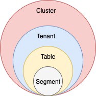
Table
Thinking of the storage, a table is the logical component that represents a collection of related records. For example, we can store a collection of e-commerce orders in the orders table, sensors readings in the readings table.
As the user, the table is the only logical component that you’ll have to deal with directly.
Schema
Each table in Pinot is associated with a Schema. A schema defines what fields are present in the table along with the data types. As opposed to RDBMS schemas, multiple tables can be created in Pinot (real-time or batch) that inherit a single schema definition.
Segments
A table is expected to grow unlimited in size. Pinot is designed to store a single table across multiple servers. To make that easier, we break a table into multiple chunks called segments. Each segment holds a subset of the records belonging to a table.
A segment is the centerpiece in Pinot’s architecture which controls data storage, replication, and scaling. Segments are physical structures that have a defined location and an address inside a Pinot cluster.
Tenants
A table is associated with a tenant. All tables belonging to a particular logical namespace are grouped under a single tenant name and isolated from other tenants.
For example, marketing and engineering can be considered as two different tenants. Tables tagged with marketing will be isolated from engineering.
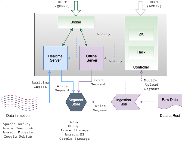
Components of a Pinot cluster
As mentioned above, A Pinot cluster is made of multiple components, each playing a unique role while in operation. Let’s explore them in detail:
Apache Zookeeper
Zookeeper is not a part of Pinot. But Pinot relies on Zookeeper for cluster management, metadata and configuration management, and coordination among different components.
Pinot Controller
You access a Pinot cluster through the Controller, which manages the cluster’s overall state and health. The Controller provides RESTful APIs to perform administrative tasks such as defining schemas and tables. Also, it comes with a UI to query data in Pinot. Controller works closely with Zookeeper for cluster coordination.
Pinot Broker
Brokers are the components that handle Pinot queries. They accept queries from clients and forward them to the right servers. They collect results from the servers and consolidate them into a single response to send it back to the client.
Pinot Server
Servers host the data segments and serve queries off the data they host. There are two types of servers — offline and real-time.
Offline servers typically host immutable segments. They ingest data from sources like HDFS and S3. Real-time servers ingest from streaming data sources like Kafka and Kinesis.
Let’s see them in action
Now that we have learned each Pinot component in detail. Let’s create a local Pinot cluster with Docker to see them in action.
We will first build a single Docker container with the latest Pinot release, start all components inside that container, ingest some data, and query them using the query console.
Let’s get started.
Before we begin
Make sure that you have Docker installed on your machine.
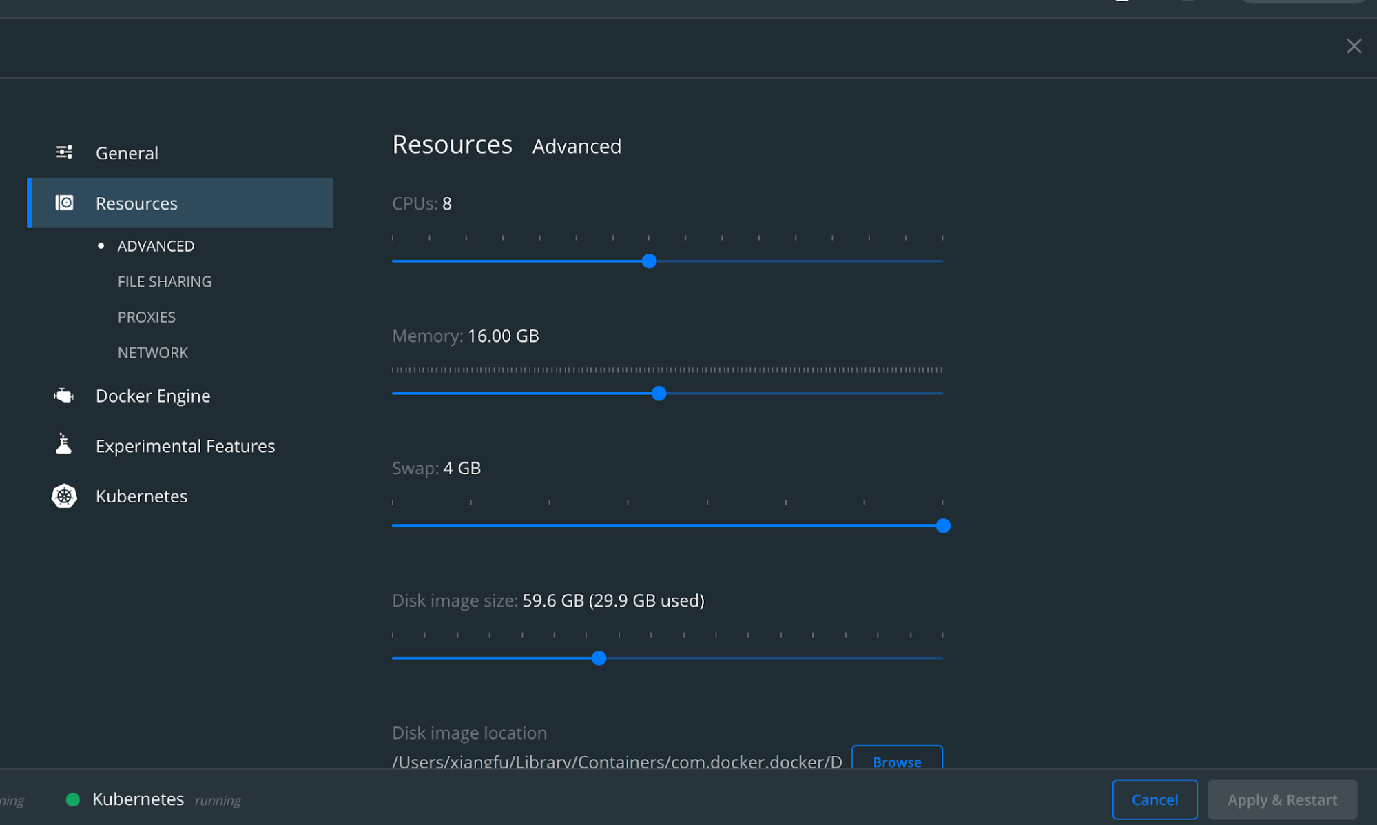
Also, allocate sufficient resources to your Docker cluster for smooth performance of Pinot. Below is a sample configuration.
Create the Dockerfile
Apache Pinot distribution comes with a launcher script called ‘quick-start-batch’, which will spin up all the components inside a single JVM. In addition to that, it will automatically create a schema and a table for a sample baseball score data set so that you can query straightaway.
Batch quickstart is ideal if you want to scratch the surface of Pinot quickly. But, in this guide, we will set up a local Pinot cluster closer to a distributed cluster. We will start each component individually so that you will be familiar with their configurations and usage as well.
First, we will create a Docker container with the latest released Pinot distribution.
Use your favorite text editor to create a Dockerfile with the following content.
    FROM openjdk:11
    WORKDIR /app
    ENV PINOT_VERSION=0.8.0
    RUN wget https://downloads.apache.org/pinot/apache-pinot-$PINOT_VERSION/apache-pinot-$PINOT_VERSION-bin.tar.gz
    RUN tar -zxvf apache-pinot-$PINOT_VERSION-bin.tar.gz
    EXPOSE 9000
    Code language: PHP (php)
In the above file, we download the latest released version of Apache Pinot (0.8.0 as of this writing) into the container and extract it. Also, the port 9000 is exposed from the container because we need to access the query console that runs inside it.
Once the Dockerfile is in place, execute the following command in a terminal window to build a Docker image and tag it as gs-pinot. Make sure that you are in the same directory as the Dockerfile is located.
docker build . -t gs-pinotThe build process will take some time. Once it is completed, let’s spin up a new container with our newly created image as follows.
docker run -p 9000:9000 -it gs-pinot /bin/bashStart Pinot components
Now that our container is up and running. Also, the last command above gave us a terminal session into the running container.
Let’s see what’s inside our working directory.
    root@06ec0a4e09c5:/app# ls
    apache-pinot-0.8.0-bin apache-pinot-0.8.0-bin.tar.gz
    Code language: PHP (php)
You can see the downloaded Pinot distributed as well as the extracted directory inside the /app directory. Let’s rename the extracted distribution as pinot.
mv apache-pinot-0.8.0-bin pinotCode language: CSS (css)The pinot directory contains different directories including bin where you can find the launcher scripts to start the Pinot cluster. The examples directory contains several quickstart samples where you can play around with as well.
Inside the bin directory, you can find the pinot-admin.sh script, which you can use to start different Pinot components. If you execute it without any arguments, it will list all the available commands. In our example, we will only use the StartZookeeper, StartController, StartBroker, and StartController commands and skip the rest. Each command has the option to specify parameters including the port, etc, but we will stick to the default ports for this demo.
Let’s start with the first component, Apache Zookeeper, which serves as the metadata storage.
Go inside the bin directory on a terminal and execute the following.
./pinot-admin.sh StartZookeeper &Note the & at the end of the command as we are running each command in the background. That will output the logs into the same terminal session.
Once we have Zookeeper up and running, we can start the controller next:
./pinot-admin.sh StartController &When the Controller starts up, it will communicate with Zookeeper to register itself. Also, it will open port 9000 so that we can access its UI later.
Now, go ahead and start the rest of the components as follows.
    ./pinot-admin.sh StartBroker &
    ./pinot-admin.sh StartServer &
It is a bit hard to believe, but now we have a Pinot cluster up and running inside a single container
Pretty neat, isn’t it?
Now let’s go ahead and type this URL in a browser window to see the Pinot UI:
http://localhost:9000
In the first screen, the UI displays the instance count for each component. If you spin up more components, the UI will be updated. By clicking on the Query Console , you will be taken to the Pinot data explorer where you can interactively query Pinot tables.
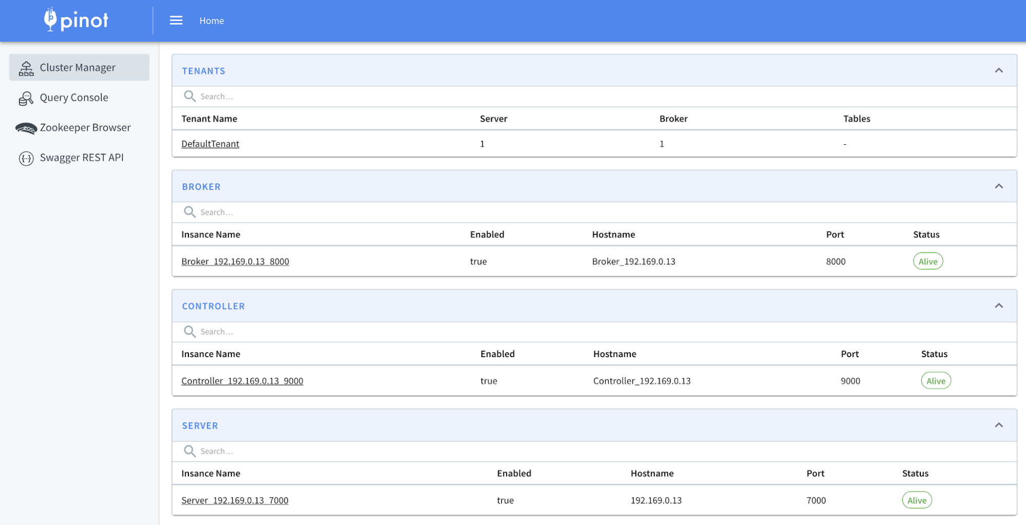
Figure 04 – Pinot data explorer runs at port 9000
You can find more information about the Pinot UI by visiting here.
Now we have a complete Pinot cluster. Let’s create a schema and table then ingest some data into that.
Create the baseballStats schema
In this section, we will ingest the baseball stats data set that you can find inside the examples/batch/baseballStats directory. This directory contains the required schema and table definition along with the raw data set.
Pinot requires you to create a schema and a table before ingesting raw data. That way, Pinot can keep track of the fields and data types of the data set to perform faster queries.
Let’s first create the schema.
Type in the following to open a new terminal session into our Pinot container. We will keep the previous session intact so that the cluster keeps running there.
First, run docker ps and get the container ID for gs-pinot to be used in the following command.
docker exec -it <CONTAINER_ID> /bin/bashCode language: HTML, XML (xml)Let’s go ahead and install vim to make it easier to edit text.
apt-get install vimCode language: JavaScript (javascript)Before creating the schema, let’s examine it first. Go inside the bin directory and open the schema definition with vim.
vim ../examples/batch/baseballStats/baseballStats_schema.jsonThat will bring in a JSON structurer like this:
{
  "metricFieldSpecs": [
    { "dataType": "INT", "name": "playerStint" },
    { "dataType": "INT", "name": "numberOfGames" },
    { "dataType": "INT", "name": "numberOfGamesAsBatter" },
    { "dataType": "INT", "name": "AtBatting" },
    { "dataType": "INT", "name": "runs" },
    { "dataType": "INT", "name": "hits" },
    { "dataType": "INT", "name": "doules" },
    { "dataType": "INT", "name": "tripples" },
    { "dataType": "INT", "name": "homeRuns" },
    { "dataType": "INT", "name": "runsBattedIn" },
    { "dataType": "INT", "name": "stolenBases" },
    { "dataType": "INT", "name": "caughtStealing" },
    { "dataType": "INT", "name": "baseOnBalls" },
    { "dataType": "INT", "name": "strikeouts" },
    { "dataType": "INT", "name": "intentionalWalks" },
    { "dataType": "INT", "name": "hitsByPitch" },
    { "dataType": "INT", "name": "sacrificeHits" },
    { "dataType": "INT", "name": "sacrificeFlies" },
    { "dataType": "INT", "name": "groundedIntoDoublePlays" },
    { "dataType": "INT", "name": "G_old" }
  ],
  "dimensionFieldSpecs": [
    { "dataType": "STRING", "name": "playerID" },
    { "dataType": "INT", "name": "yearID" },
    { "dataType": "STRING", "name": "teamID" },
    { "dataType": "STRING", "name": "league" },
    { "dataType": "STRING", "name": "playerName" }
  ],
  "schemaName": "baseballStats"
} Code language: JSON / JSON with Comments (json)
This schema file contains all the metrics, dimensions, and timestamp columns that the table is going to implement. Pay close attention to different dimensions like playerID, teamID, and league that describe the data set. Also, you can perform aggregations over metrics like runs, hits, etc.
In the new terminal session, execute the following command to add the schema into Pinot.
./pinot-admin.sh AddSchema -schemaFile ../examples/batch/baseballStats/baseballStats_schema.json -execOnce it is completed, go to the Pinot UI and check under the Zookeeper Browser as follows. You can see the baseballStats schema has been added to the property store.
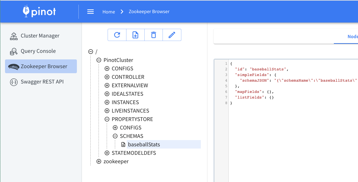
Figure 05 – Zookeeper browser keeps metadata about schemas and tables.
Create the baseballStats table
Now that we have our schema defined. Let’s create a table as well.
Let’s see how the table definition would look.
Open the table definition file from the same location.
vim ../examples/batch/baseballStats/baseballStats_offline_table_config.jsonThat will bring in a JSON structure like this:
        {
            "tableName":"baseballStats",
            "tableType":"OFFLINE",
            "segmentsConfig":{
                "segmentPushType":"APPEND",
                "segmentAssignmentStrategy":"BalanceNumSegmentAssignmentStrategy",
                "schemaName":"baseball",
                "replication":"1"
            },
            "tenants":{},
            "tableIndexConfig":{
                "loadMode":"HEAP",
                "invertedIndexColumns":[
                    "playerID",
                    "teamID"
                ]
            },
            "metadata":{
                "customConfigs":{}
            }
        }
    Code language: JSON / JSON with Comments (json)
At a very high level, this table definition contains the following information.
- How Pinot should create segments for this table
- Required indexing configurations
- Table type, which is set to OFFLINE in this case
We will talk about these in a future blog post in detail.
Type in the following command to create the baseballStats table.
    ./pinot-admin.sh AddTable
    -tableConfigFile ../examples/batch/baseballStats/baseballStats_offline_table_config.json -exec
Once you do that, go to the Pinot UI and check under the Tables section. You will find the baseballStats table along with its schema definition.
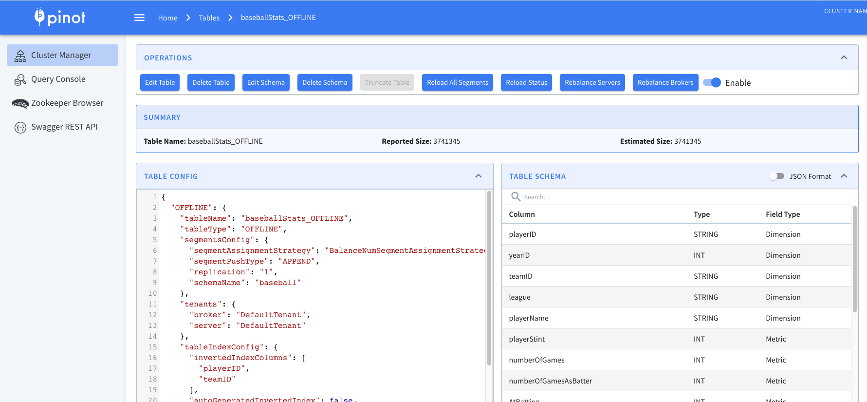
Figure 06 – Table configuration and the schema definition for baseballStats
Create an ingestion job
If you click on the baseballStats table in the query console, you will see an empty table. That is because we haven’t ingested any data yet.
In order to ingest data, Pinot requires you to create an ingestion job specification file. This file tells Pinot about where to find the raw data, where to create the segments, and other configuration directives related to the ingestion.
Let’s open the job specification from the same location as before.
vim ../examples/batch/baseballStats/ingestionJobSpec.yamlPay close attention to inputDirURI and outputDirURI attributes. Their values must contain the absolute paths. To make it easier for this example, let’s copy the job specification file into the /app directory as job.yml and refer to that location from the specification.
Now change the values as follows.
    inputDirURI: 'app/pinot/examples/batch/baseballStats/rawdata'
    outputDirURI: 'app/pinot/examples/batch/baseballStats/segments'
    Code language: JavaScript (javascript)
Once it is done, execute the following command in the terminal to create the ingestion job. We will be using the pinot-admin script again, but with a different command this time.
    ./pinot-admin.sh LaunchDataIngestionJob
    -jobSpecFile /app/job.yml
Our data set is small in size. So you should see the job completed quickly. Go ahead and check the baseballStats table in the query console again. This time, you should see data inside it.
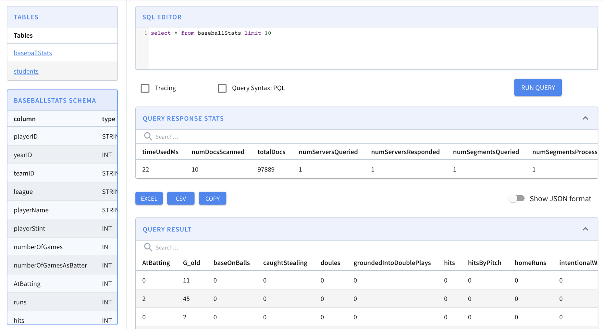
Figure 07 – baseballStats table with data
The console is good enough to automatically load the first 10 records once you click on the table name. As you can see, we have ingested 97889 records in total.
Now let’s write an analytical query to find out which team has scored the most home runs. Type in the following query into the console and press enter.
    SELECT teamID, sum(homeRuns)
    FROM baseballStats
    GROUP BY teamID
    ORDER BY sum(homeRuns) DESC
    LIMIT 10
The results will show you that New York has the most home runs. If you are into baseball, that must be obvious, isn’t it?
Where next?
In this post, you learned the logical concepts associated with Pinot as well as the different components that make a Pinot cluster. Then we managed to spin up all components in a single container which is acceptable for a demo like this but not recommended for a production environment.
We defined a schema and a table for the baseball stats data set because Pinot expects the shape of the data arriving beforehand. Once the schema and the table are in place, we created an ingestion job to ingest the raw data set into Pinot.
To conclude, we ran a SQL query against the ingested data set to find out which team has scored the most home runs.
More resources:
- See our upcoming events: https://www.meetup.com/apache-pinot
- Follow us on Twitter: https://twitter.com/startreedata
- Subscribe to our YouTube channel: https://www.youtube.com/startreedata