Introduction To Geospatial Queries In Apache Pinot

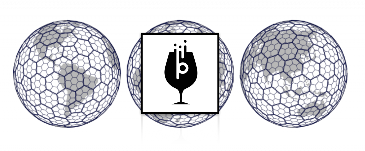
Image credits: Visualizing City Cores with H3, Uber’s Open Source Geospatial Indexing System
Geospatial data has been widely used across the industry, spanning multiple verticals, such as ride-sharing and delivery, transportation infrastructure, defense and intel, public health. Deriving insights from timely and accurate geospatial data could enable mission-critical use cases in the organizations and fuel a vibrant marketplace across the industry. In the design document for this new Pinot feature, we discuss the challenges of analyzing geospatial at scale and propose the geospatial support in Pinot.
To get started with this feature in 0.7.1, you will need to use a transform function in your schema definition configuration for a table.
The first thing you will need to add to your schema definition file to enable geolocation-based queries is your latitude and longitude fields. These fields will be imported from your data source, either from an offline data source or streaming.

A snippet defining latitude and longitude fields from a primary data source
In your list of fields, which are either imported by their unique name or generated during ingestion using a transform function, you’ll need to list both latitude and longitude fields, as shown above (lon, lat). There is nothing too special going on here, but you’ll need to generate a new field to execute real-time geospatial queries on these fields. You’ll need to generate a new field, which I’ve named location_st_point in the snippet below.
FYI — both of these snippets are from the same configuration block in your schema definition file.

A snippet of a generated field in a schema definition for geospatial querying
Now that we’ve added the necessary bits to the schema configuration file, we can now move on to updating the table configuration that references the above schema. The changes here are simple and can be seen below. There may be some changes in future versions, so it’s always good to head over to the most recent version of the Apache Pinot documentation.
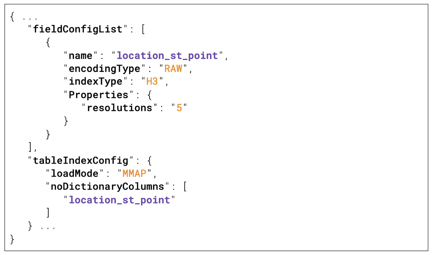
The final step to enable geospatial indexing is to modify your table config with the settings shown above.
The index type for location_st_point is set to H3, which we will explore in depth later.
The resolutions specified in the Pinot table configuration above increase the number of unique indexes depending on the value you’ve chosen. For the value resolutions: "5", Pinot will create roughly 2,016,842 unique indexes.
You can find more information about the resolutions property from the following resource, which describes the indexing tradeoff for sparse and coarse precision at query time: Table of Cell Areas for H3 Resolutions
After you’ve created both your schema and table in Pinot using the above configurations, you’ll be able to start ingesting and indexing geospatial data using H3 under the hood and start executing queries in real-time. In the next section, we’ll dive deeper into what H3 indexing is and why it makes geospatial queries so fast in Apache Pinot.
Understanding Geospatial Queries in Pinot
The geospatial implementation in Pinot relies on an open source project that originated at Uber called H3. As most users or drivers for Uber or UberEats know, their entire business relies heavily on analyzing the distance between riders, drivers, restaurants, and food delivery locations in the spatial geometry of the real world. This required an innovative solution for real-time geospatial queries at ultra-scalable demands. To respond to this challenge, engineers at Uber created a solution called the Hexagonal Hierarchical Geospatial Indexing System or H3 for short.
The basic idea is that all locations within an approximate hexagonal distance from a center point will be returned as a result when a query completes. That seems rather simple at face value, but the challenge of performant indexing for real-time OLAP queries requires a higher dimensional method for grouping sets of points. This is why H3 uses hexagonal tessellation (tiling) to optimally group sets of geospatial coordinates for scalable geospatial indexing.
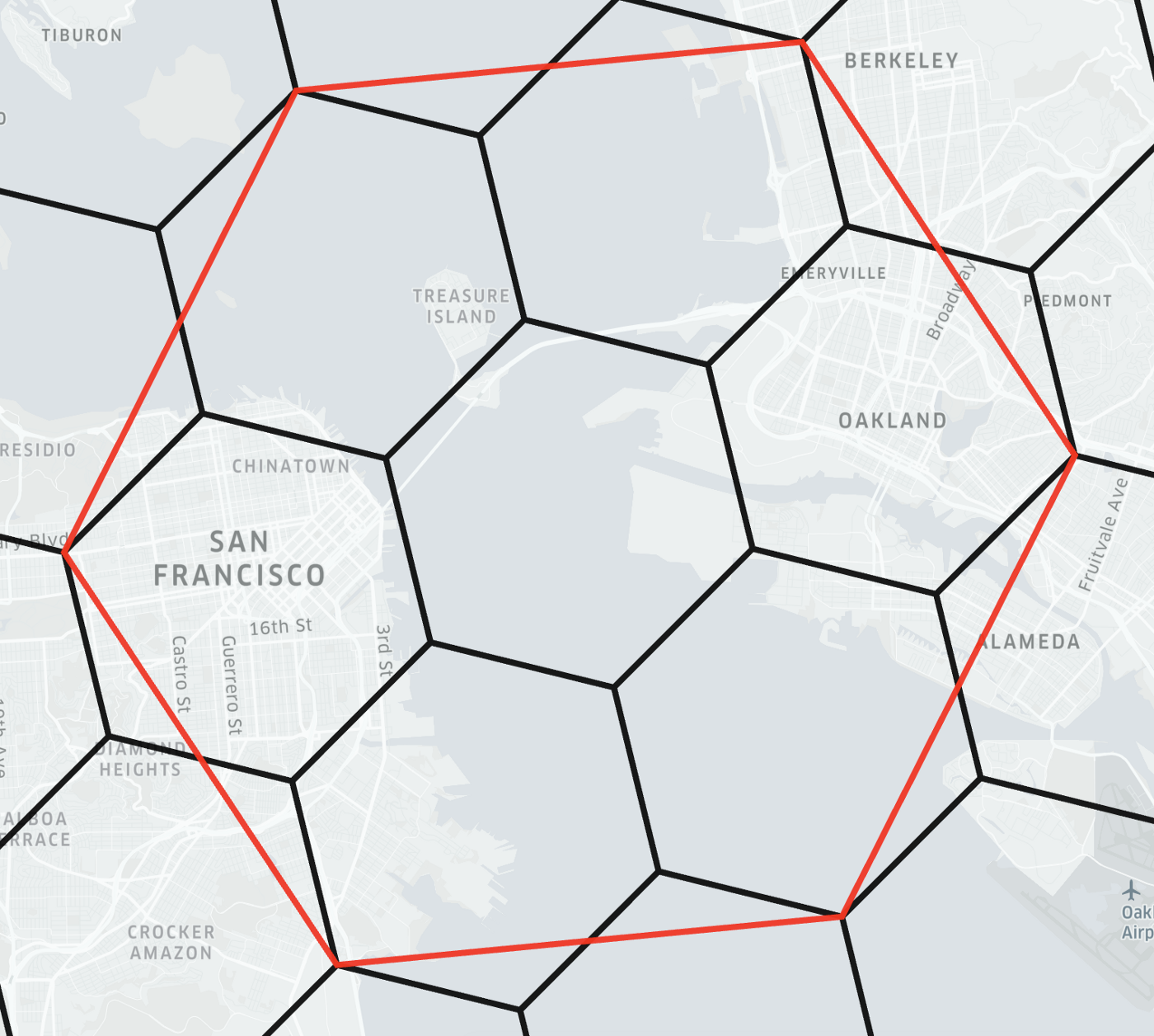
Image credits: https://h3geo.org/docs/highlights/indexing/
Documentation resources for H3 and its Apache Pinot implementation can be found at the following links:
Geospatial SQL Queries in Apache Pinot
In the Apache Pinot query shown below, we have a simple SQL lookup to find Starbucks store locations in the SF Bay Area. The center point is defined in this query using Pinot’s ST_POINT(x,y,isGeometry) function.

Return all Starbucks locations within 5km of the specified point in the SF Bay Area.
In the query, you can see that the function ST_POINT has three parameters. The third parameter is a boolean value which represents whether or not the center point for this distance query should be measured using geometry or geography. The Pinot documentation explains in-depth about how geometry and geography play a role in defining geospatial coordinates. You can also find a reference to the source code for its implementation here.
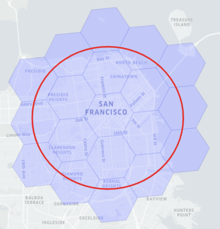
Image credits: https://h3geo.org/docs/highlights/indexing/
Why Hexagons?
The image below shows an example of how hexagons can be uncompacted and compacted, which is at the heart of the indexing technique employed by H3. Where there are many dense coordinates compacted geographically in small areas, such as is the case within big cities like San Francisco, the resolution of hexagon boundaries can be increased in number.
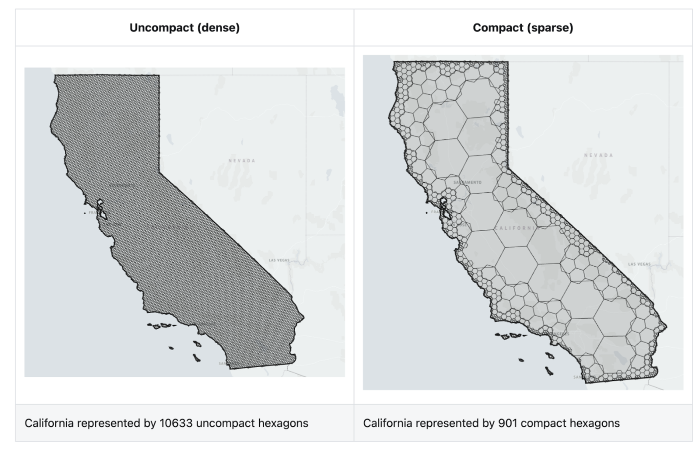
Image credits: https://h3geo.org/docs/highlights/indexing/
In the opposite scenario, there is likely not going to be a lot of interesting things in places like the interior of the Mojave Desert in Southern California, which is why we see large sparse hexagons in that area. The hexagons overlay one another in the compacted scenario, which is a kind of hierarchical index, which is the most common type of indexing technique for database technologies (such as a B-tree).
H3 Geospatial Indexing Resources
There are several great resources to learn more about how H3 geoindexing works under the hood. I highly recommend this observable notebook that explores how compacting works for the differing values for the resolutions property in a Pinot table configuration.
To understand the indexing tradeoffs for resolutions using H3 indexing, take a look at the following table resource.
There is also an excellent interactive Observable example that explains the basics of H3, which is well worth a look for those that are new to this kind of geospatial indexing.
Finally, here is a great presentation from the Uber open source team that introduces you to H3 and geoindexing.
Special thanks
It’s a pleasure to be able to explore the amazing work of the Apache Pinot committers that make these features possible. I would like to thank Yupeng Fu for co-authoring this blog post with me. His work on the design documentation is a work of art and got me excited about this new feature for Pinot.
Many thanks to the engineers and data scientists at Uber that open sourced both their code on H3 as well as their design philosophies.
If you have any questions about implementing geospatial indexing in your Pinot application, please feel free to reach out here or on our community Slack channel.
Additional learning resources
Download page: https://pinot.apache.org/download/
Getting started: https://docs.pinot.apache.org/getting-started
Join our Slack channel: https://communityinviter.com/apps/apache-pinot/apache-pinot
See our upcoming events: https://www.meetup.com/apache-pinot
Follow us on Twitter: https://twitter.com/startreedata
Subscribe to our YouTube channel: https://www.youtube.com/startreedata
Apache Pinot